我制作的工程代码在这:Tiny_Face_Recognition
之前的人脸识别效果不好,直接导致后续的其他的工作效果不好,于是寻找到现有的一个非常良心的论文,和我的数据集用的基本一致,而且效果非常的好。于是定了一个一周计划去复刻,每天以博文的形式记录。
开始之前先说一下我之前的人脸识别的步骤,我在学习Siamese Network时直接参考了one-shot Face Recognition的相关论文,所以直接搭建了Siamese ResNet152进行人脸的相似度网络。这样识别的时候,先扔进去一张自己的照片,再扔别的照片的时候可以通过人脸特征的相似度匹配,识别出是/还是不是你的照片。但准确率没有90%,还存在很多的问题。
所以开始这篇论文的学习,刚好他用的数据集和验证集和我的一样,正好可以参考他的进行搭建,实现一个正常的人脸识别的流程。
论文地址:https://arxiv.org/abs/1801.07698
参考代码地址(使用的MXNet):https://github.com/deepinsight/insightface#512-d-feature-embedding
训练集:MS-Celeb-1M
验证集:LFW
相关预知识
Softmax Loss
Softmax 公式:
\[S_j = \frac{e^{a_j}}{\sum_{i=1}^{N}{e^{a_i}}}\]其中$a_j$表示FC层向量a中某一位置(类别)j的数值,分母表示所有类别累加,实质上表示取得某个类别的概率。
Softmax Loss 公式:
\[L_{softmax} = -\sum_{j=1}^{N}{y_{j}*log(s_j)}\]其中$y_j$表示分类的标签值,在N个中只有1个为1,别的都为0,实质上这个公式就等于$L = -log(s_j)$,反向传播的时候,直接对输入求导,比较简单,直接梯度下降就可以更新参数了,这里就不多赘述。
Center Loss
Center Loss 函数:
\[L_{center} = \frac{1}{2}\sum_{i=1}^{N}{\|x_i-C_{y_i}\|^2}\]其中$C_{y_i}$表示第$y_i$类别的特征中心,反向传播的时候会随着提取特征变化而变化,训练的时候同一类会靠近特征中心。
Total Loss函数就是softmax loss和center loss加权加到一起:
\[L = L_s + \lambda L_c\]为什么要加到一起?
Softmax Loss是最大化不同类别间的差异,类内的差异是有很大的变化。
Center Loss是最小化同类间的距离,类内差异最小。
两者结合达到了联合监督的效果。
为什么比较适用于人脸?
普通场景的分类中,所有的类别都是知道的(closed-set),直接可以Softmax达到比较好的效果。
人脸中,测试集中的人某个可能没有出现在训练集过(open-set),所以希望在训练的时候能达到 类内紧凑(同一个人intra-class compactness) 类间分离(不同的人inter-class discrepancy)
Triplet Loss
这个loss有三个输入:一个图像A,一个和A同一个人的样本图像B,一个和A不同人的样本图像C
不等式关系:
\[\|x_i^a - x_i^p\| + threshold < \|x_i^a - x_i^n\|\]其中$x_i^a$表示标准图像,$x_i^p$表示同类样本,$x_i^n$表示不同类样本。意思非常的简单,同类的东西的距离加上阈值,也一直小于不同类样本的距离。
Triplet Loss公式:
\[L_{triplet} = arg\min{\sum_i{\|x_i^a - x_i^p\| + threshold - \|x_i^a - x_i^n\|}}\]它的目标也很简单,就是拉近a和p之间的距离,拉远a和n之间的距离。
关于Softmax Loss和Triplet Loss的缺点,在论文第二页中有提到,说的很清楚,我也就不翻译了:
Softmax Loss drawbacks:
- The size of the linear transformation matrix $W \in \mathbb{R}^{d\times n}$ increases linearly with the identities number n.
- The learned features are separable for the cloesd-set classification problem but not discriminative enough for the open-set face recognition problem.
Triplet Loss drawbacks:
- There is a combinatorial explosion in the number of face triplets especially for large-scale datasets, leading to a significant increase in the number of iterration steps.
- Semi-hard sample mining is a quite difficult problem for effective model training.
A-Softmax Loss
这个是对Softmax Loss的改进,比较复杂。这也是需要精度的论文之一,原始论文地址:https://arxiv.org/abs/1704.08063
原始softmax公式:
\[S_j = \frac{e^{a_j}}{\sum_{i=1}^{N}{e^{a_i}}}\]其中$a_j = W_{y_j}^{T} x_i + b_{y_j}$,W和x在这里用到的是矩阵乘法,所以引人一个角度参数$\theta$
将:
\[W_i^{T} x + b_i\]写作:
\[\|W_i^T\|*\|x\|*\cos{\theta_i} + b_i\]为什么要这样干?
原Softmax的决策边界(比如二分类的边界,得到的结果同属于两个类别,即两个概率相同,p1==p2)是:
\[p_1 = W_1^T x + b_1 == p2 = W_2^T + b_2\]即
\[(W_1 - W_2)x + b1 - b2 = 0\]引入角度后,决策边界变为:
\[\|x\|(\cos{\theta_1} - \cos{\theta_2}) == 0\]会发现,W已经没有了,只剩下了角度$\theta$
又是将在这个变换代入到原来的Softmax Loss中并取消偏置(去掉所有的b),即为Modified-Softmax Loss
很重要的是,我们还需要引入一个m去作为类别的数量,即在$\theta$前加入一个m的参数:
\[\|W_i^T\|*\|x\|*\cos{m*\theta_i}\]所以整体的A-Softmax公式为:
\[L_{a-softmax} = \frac{1}{N} \sum_j{-\log{\frac{e^{\|x_j\|\cos{(m*\theta_{y_j}, j)}}}{e^{\|x_j\|\cos{(m*\theta_{y_j}, j)}} + \sum_{i\neq y_j}{e^{\|x_i\|\cos{(\theta_i, j)}}}}}}\]其中$\theta$的范围是[0, pi/m],为了消除这个范围,对cos还要进行扩展:
\[\psi(\theta_{y_j, j}) = (-1)^k \cos{(m\theta_{y_j, j})} - 2k\]其中:
\[\frac{k\pi}{m} <= \theta_{y_j, j} <= \frac{(k+1)\pi}{m}, 0<=k<=m-1\]用这个将cos给代替,即为真正的A-Softmax Loss
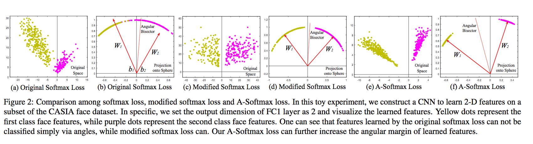
在原论文中给出了Softmax和它的几何定义,非常清晰。
介绍ArcFace
这篇论文提出了一个叫做 Additive Angular Margin Loss,即ArcFace的Loss,改进基于上面的A-Softmax。
公式为:
\[L_{arcface} = \frac{1}{N} \sum_j{-\log{\frac{e^{s(\cos(\theta_{y_j} + m))}}{e^{s(\cos(\theta_{y_j} + m))} + \sum_{i\neq y_j}{e^{scos{(\theta_i, j)}}}}}}\]具体为什么和其他的我还没看懂,明天再看。
第一天代码
原评测中效果较好的为LResNet50E-IR,其中L表示112112人脸图片,IR表示对ResNet的block进行了一些改进,所以我先搭建一个原始的224224的ResNet-50
ResNet50的结构为:(3+4+6+3)*3+2,需要四个Block块
先定义Block数据结构:
class Block(collections.namedtuple('Block', ['scope', 'unit_fn', 'args'])):
	pass
设计50层ResNet顶层函数:
def resnet_50(inputs, num_classes=None, global_pool=True, reuse=None, scope='renet_50'):

	blocks = [
		Block('block1', bottleneck, [(256, 64, 1)] * 2 + [(256, 64, 2)]),
		Block('block2', bottleneck, [(512, 128,1)] * 3 + [(512, 128, 2)]),
		Block('block3', bottleneck, [(1024, 256, 1)] * 5 + [(1024, 256, 2)]),
		Block('block4', bottleneck, [(2048, 512, 1)] * 3)
	]

	return resnet_v2(inputs, blocks, num_classes, global_pool, include_root_block=True, reuse=reuse, scope=scope)
其中包含残差函数bottleneck和resnet运行环境两部分。
残差函数bottlenect:
def bottleneck(inputs, depth, depth_bottlenect, stride, outputs_collections=None, scope=None):
	with tf.variable_scope(scope, 'bottleneck_v2', [inputs]) as sc:
		# 获取输入最后一维,即输出通道,限定min_rank最小维度为4
		depth_in = slim.utils.last_dimension(inputs.get_shape(), min_rank=4)
		# 对输入进行Batch_Normalization
		preact = slim.batch_norm(inputs, activation_fn=tf.nn.relu, scope='preact')

		if depth == depth_in:
			# 如果残差单元输入通道和输出通道一致,按照步长对inputs进行降采样
			shortcut = subsample(inputs, stride, 'shortcut')
		else:
			# 不一致就按步长和1*1卷积改变通道数,使两者一致
			shortcut = slim.conv2d(preact, depth, [1,1], stride=stride, normalizer_fn=None, activation_fn=None, scope='shortcut')

		# 输出通道为 depth_bottleneck
		residual = slim.conv2d(preact, depth_bottleneck, [1,1], stride=1, scope='conv1')

		# 输出通道为depth_bottleneck, 步长为stride, 3*3卷积
		residual = conv2d_same(residual, depth_bottleneck, 3, stride, scope='conv2')

		# 最后一层1*1卷积,步长1,输出depth的卷积,无正则,无激活函数
		residual = slim.conv2d(residual, depth, [1,1], stride=1, normalizer_fn=None, activation_fn=None, scope='conv3')

		# 将结果和降采样结果相加
		output = shortcut + residual
		# 将output加入collection并返回output作为函数结果
		return slim.utils.collect_named_outputs(outputs_collections, sc.name, output)
其中用到了降采样和卷积层两个方法
降采样方法:
def subsample(inputs, facor, scope=None):
	if factor == 1:
		return inputs
	else:
		return slim.max_pool2d(inputs, [1, 1], stride=factor, scope=scope)
创造卷积层:
def conv2d_same(inputs, num_outputs, kernel_size, stride, scope=None):
	if stride == 1:
		return slim.conv2d(inputs, num_outputs, kernel_size, stride=1, padding='SAME', scope=scope)
	else:
		# 显式的pad zero总数为kernel_size - 1
		pad_total = kernel_size - 1
		pad_beg   = pad_total // 2
		pad_end   = pad_total - pad_beg
		# 对输入进行补0
		inputs = tf.pad(inputs, [[0, 0], [pad_beg, pad_end], [pad_beg, pad_end], [0, 0]])
		return slim.conv2d(inputs, num_outputs, kernel_size, stride=stride, padding='VALID', scope=scope)
最后是resnet运行环境:
def resnet_v2(
	inputs, # 输入 [batch, height, weight, channels]
	blocks, # 多个['scope', 'unit_fn', 'args']
	num_classes=None,  # 最后输出类数
	global_pool=True,  # 是否最后进行平均池化
	include_root_block=True, # 是否在最前面加上7*7卷积和最大池化
	reuse=None,    # 是否重用
	scope=None     # 名称
):
	with tf.variable_scope(scope, 'resnet_v2', [inputs], reuse=reuse) as sc:
		# 定义end_points_collection
		end_points_collection = sc.original_name_scope + '_end_points'
		# 将三个参数的outputs_collections默认设置为end_points_collection
		with slim.arg_scope([slim.conv2d, bottleneck, stack_blocks_dense], outputs_collections=end_points_collection):
			net = inputs
			if include_root_block:
				with slim.arg_scope([slim.conv2d], activation_fn=None, normalizer_fn=None):
					# 64输出通道,7*7卷积
					net = conv2d_same(net, 64, 7, stride=2, scope='conv1')
				# 接最大池化
				net = slim.max_pool2d(net, [3, 3], stride=2, scope='pool1')
			# 生成残差学习模块
			net = stack_blocks_dense(net, blocks)
			net = slim.batch_norm(net, activation_fn=tf.nn.relu, scope='postnorm')

			if global_pool:
				# 全局平均池化层
				net = tf.reduce_mean(net, [1,2], name='pool5', keep_dims=True)
			if num_classes is not None:
				# 是否有通道数
				net = slim.conv2d(net, num_classes, [1, 1], activation_fn=None, normalizer_fn=None, scope='logits')
			# 转化collection到python的dict
			end_points = slim.utils.convert_collection_to_dict(end_points_collection)

			# Softmax激活,输出网络结果
			if num_classes is not None:
				end_points['predictions'] = slim.softmax(net, scope='predictions')

			return net, end_points
其中包含arg_scope和stack_blocks_dense,具体实现如下
arg_scope, 定义参数默认值:
def resnet_arg_scope(
	is_training=True,       # 是否训练
	weight_decay=0.0001,    # 权重衰减速率
	batch_norm_decay=0.997, # BN衰减速率
	batch_norm_epsilon=1e-5, # BN的epsilon默认值
	batch_norm_scale=True    # BN的scale默认值
):
	batch_norm_params = {
		'is_training': is_training,
		'decay': batch_norm_decay,
		'epsilon': batch_norm_epsilon,
		'scale': batch_norm_scale,
		'updates_collections': tf.GraphKeys.UPDATE_OPS,
	}

	with slim.arg_scope(
		[slim.conv2d],
		weights_regularizer = slim.l2_regularizer(weight_decay),
		weights_initializer = slim.variance_scaling_initializer(),
		activation_fn = tf.nn.relu,
		normalizer_fn = slim.batch_norm,
		normalizer_params = batch_norm_params)
		):
		with slim.arg_scope([slim.batch_norm], **batch_norm_params):
			with slim.arg_scope([slim.max_pool2d], padding='SAME') as arg_sc:
				return arg_sc # 最后将基层嵌套的arg_scope作为结果返回

}
stack_blocks_dense,堆叠Blocks的函数
def stack_blocks_dense(net, blocks, outputs_collections=None):
	# 两层循环,逐个Residual unit堆叠
	for block in blocks:
		with tf.variable_scope(block.scope, 'block', [net]) as sc:
			for i, unit in enumerate(block.args):
				# 第二层循环展开四个参数
				with tf.variable_scope('unit_%d' % (i+1), values=[net]):
					unit_depth, unit_depth_bottleneck, unit_stride = unit
					# 使用残差学习单元的生成函数顺序的创建并连接所有的残差学习单元
					net = block.unit_fn(net, depth=unit_depth, depth_bottleneck=unit_depth_bottleneck, stride=unit_stride)
			net = slim.utils.collect_named_outputs(outputs_collections, sc.name, net)
	# 所有Block的residual unit都堆叠完之后,再返回net作为stack_blocks_dense
	return net