我制作的工程代码在这:Tiny_Face_Recognition
除了熟知的CNN中的卷积层外,一个略微完整的人脸识别的流程还有很多特殊的层,今天主要把这些特殊的层给记录清楚,原文中评测值最高的是SE-LResNet50E-IR,当然我没有用SE,因为还不知道是什么意(这几段在新版中没有具体说明,只能找最初的论文),所以今天主要把这些特殊的层研究一下。
按照BN->LRes的L->50E的E->IR->SE的顺序来。
ArcFace论文:https://arxiv.org/abs/1801.07698
BN论文:https://arxiv.org/abs/1502.03167
Batch Normalization
原始论文在15年提出:https://arxiv.org/abs/1502.03167
这个东西可以看到出现的量很大,它有什么作用?主要作用就三个:
- 降低Internal Covariate Shift,也就是当输入的分布进行改变的时候,尽量不妨碍网络的结果。
- 加快训练速度。
- 防止Gradient Vanishing和Exploding
对第一个的解释就是,一个前向传播的例子是$y=W\cdot x$,要进行学习的是$W$,那么在$x$的分布非常不均衡,极端的情况下,比如$x_1=1, x_2=100$,那么可能发生什么,这里借用李宏毅老师的图来看看:

左边可以看到$W_1$对$W_2$的影响是比较小的,而$W_2$对$W_1$的影响很大,整个Loss呈现一个椭圆,而如果$x_1$和$x_2$的差别进一步放大的话(这种情况其实是比较常见的),就会压缩的越瘪,在不同的地方Learning rate还要不一样,就会非常的麻烦。所以我们希望$x$整体能有一个比较正常的分布,至少都在一个Range里面。一般的方法就是做一个Norm即可。
对第二个的解释就是,BatchNorm了之后,我们可以使用稳定的比较大的学习率,这样自然就提高了训练的速度。
对第三个的解释先放着,先说BN的原理。
这时候就需要放一张用烂了的原始论文中的一张图:

要注意的是BN的输入这个$x_i$并不是一个Batch中的原始的数据,而是BN作为一个层,一个Layer的输入,也就是是经过了$W\cdot x$之后的输出。
然后对算这一套$x$的均值和方差,再做一个N(0,1)的normalization操作。
最后需要注意的就是最后引入了两个学习参数,一个$\gamma$和一个$\beta$,这两个是BN层中需要训练的参数,引入它们的原因就是加入一个保险装置,可以看到如果$\gamma == \sigma, \beta == \mu$的时候,就等于没有Normalization,当然这种情况是不可能的,因为这两个参数的值和input没有关系,当然也不是说这两个参数就是常数,它们的值是学习得到的。
在进行Train的时候,$\mu$和$\sigma$都是通过一整个Batch计算得来的,但是在Test的时候,你没有一个Batch,你就一个数据,怎么得到$\mu$和$\sigma$呢?这种时候有两种做法:
- 用整个Training dataet的$\mu$和$\sigma$代替,但有很严重的问题,就是Training dataset过大,还有一些别的问题,所以主要用第二种方法。
- 把过去的$\mu$和$\sigma$每次更新的值都摸出来做一个Average,但也有问题,就是整个更新的生存期中,它们的差值也是很大的,比如刚开始的时候比较小,后来比较大的情况等等。
那么回到之前的好处,为什么可以防止Gradient Vanishing和Exploding?
这一篇讲的就很好,引用一下:https://www.zhihu.com/question/38102762/answer/164790133
首先看一下产生的原因。
前向传播的时候,$h_l = {w_l}^T h_{l-1}$
l层的值由前一层和参数变换得到,那么反向传播的时候,求偏导:
\[\frac{\partial l}{\partial h_{l-1}} = \frac{\partial l}{\partial h_{l}} \frac{\partial h_l}{\partial h_{l-1}} = \frac{\partial h_l}{\partial h_{l}} W_l\]要多来几层的话,反向传播就会乘好多个W,比如从l层到k层:
\[\frac{\partial l}{\partial h_{k}} = \frac{\partial l}{\partial h_{l}} \prod _{i=k+1}^{l}{w_i}\]如果有100层,w假设是0.9,那么$0.9^100=0.00005$了,所以就Gradient Vanshing了,同理如果w假设是1.1,那么就会爆炸,就Gradient Exploding了。
BN在这里面起到了怎样的作用?
加了BN之后,BN每一次更新$W$的时候,都会进行一次$1/\alpha$的操作,它不会妨碍到继续的计算。
接下来看一下BN层实现,继承的是TensorLayer,大体的步骤就是:
- 初始化层内参数$\beta, \gamma$
- 算均值和方差
- 如果是训练步骤的话,更新均值和方差,调用tf.nn.batch_normalization,传入均值方差和两个参数
- 如果是测试步骤的话,计算之前的均值和方差的均值,传入tf.nn.batch_normalization即可。
tips: epsilon的是个很小的值,主要是用来防止var为0的情况
代码如下,来源与说明均在注释:
class BatchNormLayer(Layer):
    """
    The :class:`BatchNormLayer` class is a normalization layer, see ``tf.nn.batch_normalization`` and ``tf.nn.moments``.
    Batch normalization on fully-connected or convolutional maps.
    ```
        https://www.tensorflow.org/api_docs/python/tf/cond
        If x < y, the tf.add operation will be executed and tf.square operation will not be executed.
        Since z is needed for at least one branch of the cond, the tf.multiply operation is always executed, unconditionally.
    ```
    Parameters
    -----------
    layer : a :class:`Layer` instance
        The `Layer` class feeding into this layer.
    decay : float, default is 0.9.
        A decay factor for ExponentialMovingAverage, use larger value for large dataset.
    epsilon : float
        A small float number to avoid dividing by 0.
    act : activation function.
    is_train : boolean
        Whether train or inference.
    beta_init : beta initializer
        The initializer for initializing beta
    gamma_init : gamma initializer
        The initializer for initializing gamma
    dtype : tf.float32 (default) or tf.float16
    name : a string or None
        An optional name to attach to this layer.
    References
    ----------
    - `Source <https://github.com/ry/tensorflow-resnet/blob/master/resnet.py>`_
    - `stackoverflow <http://stackoverflow.com/questions/38312668/how-does-one-do-inference-with-batch-normalization-with-tensor-flow>`_
    """

    def __init__(
            self,
            layer=None,
            decay=0.9,
            epsilon=2e-5,
            act=tf.identity,
            is_train=False,
            fix_gamma=True,
            beta_init=tf.zeros_initializer,
            gamma_init=tf.random_normal_initializer(mean=1.0, stddev=0.002),  # tf.ones_initializer,
            # dtype = tf.float32,
            trainable=None,
            name='batchnorm_layer',
    ):
        Layer.__init__(self, name=name, prev_layer=None)
        self.inputs = layer.outputs
        # print("  [TL] BatchNormLayer %s: decay:%f epsilon:%f act:%s is_train:%s" % (self.name, decay, epsilon, act.__name__, is_train))
        x_shape = self.inputs.get_shape()
        params_shape = x_shape[-1:]

        from tensorflow.python.training import moving_averages
        from tensorflow.python.ops import control_flow_ops

        with tf.variable_scope(name) as vs:
            axis = list(range(len(x_shape) - 1))

            ## 1. beta, gamma
            if tf.__version__ > '0.12.1' and beta_init == tf.zeros_initializer:
                beta_init = beta_init()
            beta = tf.get_variable('beta', shape=params_shape, initializer=beta_init, dtype=tf.float32, trainable=is_train)  #, restore=restore)

            gamma = tf.get_variable(
                'gamma',
                shape=params_shape,
                initializer=gamma_init,
                dtype=tf.float32,
                trainable=fix_gamma,
            )  #restore=restore)

            ## 2.
            if tf.__version__ > '0.12.1':
                moving_mean_init = tf.zeros_initializer()
            else:
                moving_mean_init = tf.zeros_initializer
            moving_mean = tf.get_variable('moving_mean', params_shape, initializer=moving_mean_init, dtype=tf.float32, trainable=False)  #   restore=restore)
            moving_variance = tf.get_variable(
                'moving_variance',
                params_shape,
                initializer=tf.constant_initializer(1.),
                dtype=tf.float32,
                trainable=False,
            )  #   restore=restore)

            ## 3.
            # These ops will only be preformed when training.
            mean, variance = tf.nn.moments(self.inputs, axis)
            try:  # TF12
                update_moving_mean = moving_averages.assign_moving_average(moving_mean, mean, decay, zero_debias=False)  # if zero_debias=True, has bias
                update_moving_variance = moving_averages.assign_moving_average(
                    moving_variance, variance, decay, zero_debias=False)  # if zero_debias=True, has bias
                # print("TF12 moving")
            except Exception as e:  # TF11
                update_moving_mean = moving_averages.assign_moving_average(moving_mean, mean, decay)
                update_moving_variance = moving_averages.assign_moving_average(moving_variance, variance, decay)
                # print("TF11 moving")

            def mean_var_with_update():
                with tf.control_dependencies([update_moving_mean, update_moving_variance]):
                    return tf.identity(mean), tf.identity(variance)
            if trainable:
                mean, var = mean_var_with_update()
                # print(mean)
                # print(var)
                self.outputs = act(tf.nn.batch_normalization(self.inputs, mean, var, beta, gamma, epsilon))
            else:
                self.outputs = act(tf.nn.batch_normalization(self.inputs, moving_mean, moving_variance, beta, gamma, epsilon))
            variables = [beta, gamma, moving_mean, moving_variance]
        self.all_layers = list(layer.all_layers)
        self.all_params = list(layer.all_params)
        self.all_drop = dict(layer.all_drop)
        self.all_layers.extend([self.outputs])
        self.all_params.extend(variables)
LRes的L
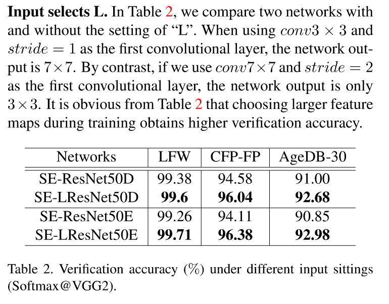
原来的ResNet做ImageNet的输入是224×224,这里的输入是112×112。
这里主要是在第一层卷积的时候用3×3的卷积核,步长为1,可以看到确实准确率高了那么一丢丢。
最后几层的option
回到原ArcFace论文中的Experimental Settings,能看到这样的一句话:
After the last convoluional layer, we explore the BN-Dropout-FC-BN stucture to get the final 512-D embedding feature.
可以看到在最后一层卷积层后,加了一个BN-Dropout-FC-BN的结构,在最后的卷积层后,这里文章作者对比了五个选项,并分别给出了结果。
- Option-A: Global Pooling Layer(GP)
- Option-B: GP + FC
- Option-C: GP + FC + BN
- Option-D: GP + FC + BN + PReLU
- Option-E: BN + Dropout + FC + BN
可以看到评测的经过如下,准确率确实又高了一丢丢:

代码中的体现就是:
net = BatchNormLayer(net, act=tf.identity, is_train=True, name='E_BN1', trainable=trainable)
net.outputs = tf.nn.dropout(net.outputs, keep_prob=keep_rate, name='E_Dropout')
net_shape = net.outputs.get_shape()
net = tl.layers.ReshapeLayer(net, shape=[-1, net_shape[1]*net_shape[2]*net_shape[3]], name='E_Reshapelayer')
net = tl.layers.DenseLayer(net, n_units=512, W_init=w_init, name='E_DenseLayer')
net = BatchNormLayer(net, act=tf.identity, is_train=True, fix_gamma=False, trainable=trainable, name='E_BN2')
其中Dense就是全连接层
IR
看上面的那个图,加了IR和不加IR的又多了一丢丢的准确率,大概0.0几左右,IR是什么?
这里是对残差块做了一个改动。
原来的残差块就两个卷积(如下图所示),现在变成了BN+Conv1+BN+PReLU+Conv2+BN,也就是说加了三个BN和一个PReLU。

当然对结果的准确率的影响就有那么一丢丢的提高。
代码来看就是这样:
shortcut = 之前算的,要么需要欠采样,要么直接是输入

residual = BatchNormLayer(inputs, act=tf.identity, is_train=True, trainable=trainable, name='conv1_bn1')
residual = BatchNormLayer(inputs, act=tf.identity, is_train=True, trainable=trainable, name='conv1_bn1')
residual = BatchNormLayer(residual, act=tf.identity, is_train=True, trainable=trainable, name='conv1_bn2')
# bottleneck prelu
residual = tl.layers.PReluLayer(residual)
residual = conv2d_same(residual, depth, kernel_size=3, strides=stride, rate=rate, w_init=w_init, scope='conv2', trainable=trainable)
SE(Squeeze and Excitation network)
这又是一篇论文提出来的东西:https://arxiv.org/abs/1709.01507
其实我没太看懂…和原来的残差单元对比的话,就是又拉出来了一条线做了几个操作

有什么好处呢?我先去网上抄一段…
- 具有更多的非线性,更好拟合通道间的复杂相关性
- 极大的减少了参数量和计算量
代码的话如下所示,主要就是在最后加了几个全连接和激活:
(ElementwiseLayer就是一个二元关系的操作,看combine_fn是什么操作就是什么关系)
# bottleneck layer 1
residual = BatchNormLayer(inputs, act=tf.identity, is_train=True, trainable=trainable, name='conv1_bn1')
residual = tl.layers.Conv2d(residual, depth_bottleneck, filter_size=(3, 3), strides=(1, 1), act=None, b_init=None,
                            W_init=w_init, name='conv1', use_cudnn_on_gpu=True)
residual = BatchNormLayer(residual, act=tf.identity, is_train=True, trainable=trainable, name='conv1_bn2')
# bottleneck prelu
residual = tl.layers.PReluLayer(residual)
# bottleneck layer 2
residual = conv2d_same(residual, depth, kernel_size=3, strides=stride, rate=rate, w_init=w_init, scope='conv2', trainable=trainable)
# squeeze
squeeze = tl.layers.InputLayer(tf.reduce_mean(residual.outputs, axis=[1, 2]), name='squeeze_layer')
# excitation
excitation1 = tl.layers.DenseLayer(squeeze, n_units=int(depth/16.0), act=tf.nn.relu,
                                   W_init=w_init, name='excitation_1')
# excitation1 = tl.layers.PReluLayer(excitation1, name='excitation_prelu')
excitation2 = tl.layers.DenseLayer(excitation1, n_units=depth, act=tf.nn.sigmoid,
                                   W_init=w_init, name='excitation_2')
# scale
scale = tl.layers.ReshapeLayer(excitation2, shape=[tf.shape(excitation2.outputs)[0], 1, 1, depth], name='excitation_reshape')

residual_se = ElementwiseLayer(layer=[residual, scale],
                               combine_fn=tf.multiply,
                               name='scale_layer',
                               act=None)

output = ElementwiseLayer(layer=[shortcut, residual_se],
                          combine_fn=tf.add,
                          name='combine_layer',act=tf.nn.relu)